Visualizing catalogs

Another way to visualize the catalogs is to plot galleries of their individual systems, where the planets in each system are plotted as points on a line along the orbital period axis (or semi-major axis). This is especially useful for looking at the multi-planet systems and their architectures.

Plotting a simple gallery

Here is a simple example using our function plot_figs_observed_systems_gallery_from_cat_obs to plot a gallery of systems with three or more observed planets.

First, load the catalogs again:

# Load modules and catalogs as before:
from syssimpyplots.general import *
from syssimpyplots.load_sims import *
from syssimpyplots.plot_catalogs import *
from syssimpyplots.compare_kepler import *

load_dir = '/path/to/a/simulated/catalog/' # replace with your path!

N_sim, cos_factor, P_min, P_max, radii_min, radii_max = read_targets_period_radius_bounds(load_dir + 'periods.out')

# Load a simulated physical catalog:
sssp_per_sys, sssp = compute_summary_stats_from_cat_phys(file_name_path=load_dir, load_full_tables=True, match_observed=True)

# Load simulated and Kepler observed catalogs:
sss_per_sys, sss = compute_summary_stats_from_cat_obs(file_name_path=load_dir)
ssk_per_sys, ssk = compute_summary_stats_from_Kepler_catalog(P_min, P_max, radii_min, radii_max)

Note

This time, we have loaded the physical catalog with the options load_full_tables=True and match_observed=True, which will include a field in sssp_per_sys containing a 2-d array indicating whether each planet is detected or not (1 or 0, respectively) in the simulation, accessible by sssp_per_sys['det_all'].

Now, pass the simulated observed catalog (sss_per_sys) into the following function as follows:

# Plot a gallery of the simulated systems with 3+ observed planets:
plot_figs_observed_systems_gallery_from_cat_obs(sss_per_sys, sort_by='inner', n_min=3, color_by='k', max_sys=50, sys_per_fig=50)
plt.show()

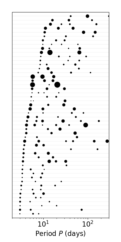
This function can be applied to both simulated observed (e.g. sss_per_sys) and Kepler-observed (e.g. ssk_per_sys) catalogs. In this example, we have selected systems with at least three observed planets (using n_max=3), sorted them by the period of their inner-most planet (using sort_by='inner'), and included 50 systems in a single figure.

Tip

You can change the number of systems, and/or the number of figures, by varying the max_sys and sys_per_fig parameters. For example, setting max_sys=200 and sys_per_fig=50 will make four figures each showing 50 different systems (if there are enough systems with the required multiplicity in the catalog).

If there are more than max_sys systems satisfying the given criteria, the function will randomly sample a subset of these systems.

The color_by parameter allows you to choose from a number of color schemes. For example, you can also color the planets by their relative size order in each system (so all the smallest planets are one color, all the 2nd smallest planets are another color, etc.):

# Plot a gallery with the planets colored by their size ordering:
plot_figs_observed_systems_gallery_from_cat_obs(sss_per_sys, sort_by='inner', n_min=3, color_by='size_order', legend=True, max_sys=50, sys_per_fig=50)
plt.show()

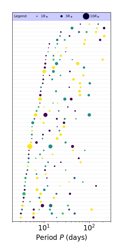
Here, we have also included a legend by setting legend=True. This gives us a reference for the relative sizes of the planets!

Sorting and labeling systems

You can also sort by planet multiplicity instead of inner-most period by setting sort_by='multiplicity', and label each system by a given quantity by setting llabel and llabel_text such as in the following example:

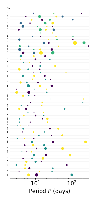
# Plot a gallery with the systems sorted and labeled by multiplicity:
plot_figs_observed_systems_gallery_from_cat_obs(sss_per_sys, sort_by='multiplicity', n_min=3, color_by='size_order', llabel='multiplicity', llabel_text=r'$n_{\rm pl}$', max_sys=50, sys_per_fig=50)
plt.show()

Tip

The label does not have to be the same as or even related to the sort_by parameter, but it’s useful for checking that it has actually sorted things correctly.

Plotting detected/undetected planets

There is a separate function for plotting galleries of physical systems, plot_figs_physical_systems_gallery_from_cat_phys. It provides much of the same functionality and uses mostly the same parameters, except it allows you to filter systems based on both the intrinsic multiplicity (using n_min and n_max) as well as the observed multiplicity (using n_det_min and n_det_max). It also contains more options for color_by, and has a mark_det boolean parameter for whether or not to indicate the detected and undetected planets. The following examples showcase some of these options:

# Plot a gallery of physical systems with at least 5 planets:
plot_figs_physical_systems_gallery_from_cat_phys(sssp_per_sys, sssp, sort_by='inner', n_min=5, n_det_min=0, color_by='cluster', mark_det=False, llabel='multiplicity', llabel_text=r'$n_{\rm pl}$', max_sys=50, sys_per_fig=50)

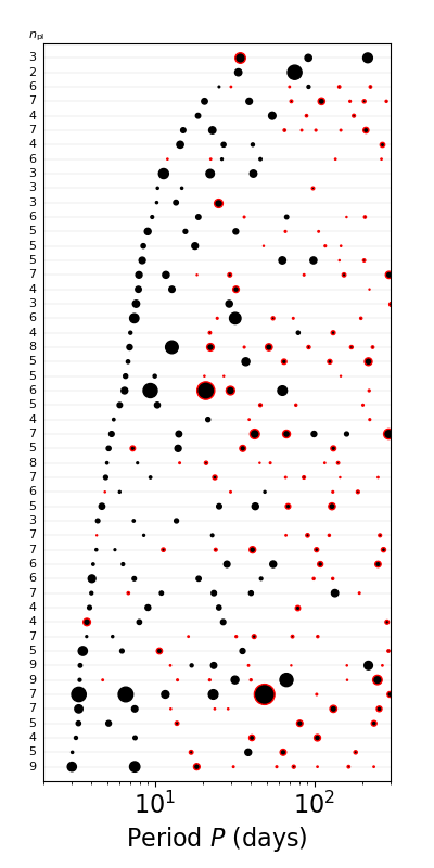
# Plot a gallery of physical systems with at least two detected planets:
plot_figs_physical_systems_gallery_from_cat_phys(sssp_per_sys, sssp, sort_by='inner', n_det_min=2, color_by='k', mark_det=True, llabel='multiplicity', llabel_text=r'$n_{\rm pl}$', max_sys=50, sys_per_fig=50)

plt.show()

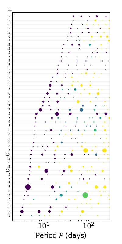
In the left figure, we selected only systems with at least five planets (regardless of whether or not any planets are detected) and colored them by their cluster id’s, so planets with the same color were drawn from the same “cluster”.

In the right figure, we selected systems with at least two detected planets and marked all undetected planets with red outlines using the mark_det=True option.

More customizations

While the two functions demonstrated above (one for plotting observed systems, another for plotting physical systems) provide many useful options for plotting galleries, you may wish to make versions of these figures that are outside the scope of what can be accomplished by these two functions. You can achieve some additional flexibility by using the function plot_figs_systems_gallery directly, which is called by both of the previous functions. For example, you may wish to plot along semi-major axes instead of orbital period for the x-axis, use planet masses instead of radii for setting the relative sizes of the points, sort the systems in a special way, provide a custom set of systems, etc… the possibilities are endless!

Other ways of plotting catalogs

There are many other functions in the syssimpyplots.plot_catalogs module for visualizing catalogs, some of which have been used to characterize other correlations in the planetary systems generated by our models.

Warning

Many of these functions are currently undocumented (they do not show up in the detailed API) and are not meant for flexible use – use them at your own risk!