Plotting histograms

A simple example

On the previous page, you learned how to load a catalog (physical and observed). These catalogs are in the form of dictionaries containing various planetary (and stellar) properties (sometimes referred to as summary statistics). One of the most basic and yet illuminating ways of visualizing a catalog is to plot histograms of the various properties. We provide several flexible functions for plotting histograms:

from syssimpyplots.general import *
from syssimpyplots.load_sims import *
from syssimpyplots.plot_catalogs import *
from syssimpyplots.compare_kepler import *

load_dir = '/path/to/a/simulated/catalog/' # replace with your path!

sss_per_sys, sss = compute_summary_stats_from_cat_obs(file_name_path=load_dir)

# To plot a histogram of the observed multiplicities (number of planets per system):
ax = plot_fig_counts_hist_simple([sss_per_sys['Mtot_obs']], [], x_min=0, x_max=8, x_llim=0.5, log_y=True, xlabel_text='Observed multiplicity', ylabel_text='Number of systems')

# To plot a histogram of the observed orbital periods:
ax = plot_fig_pdf_simple([sss['P_obs']], [], x_min=3., x_max=300., normalize=False, log_x=True, log_y=True, xticks_custom=[3,10,30,100,300], xlabel_text=r'$P$ (days)', ylabel_text='Number of planets')

plt.show()

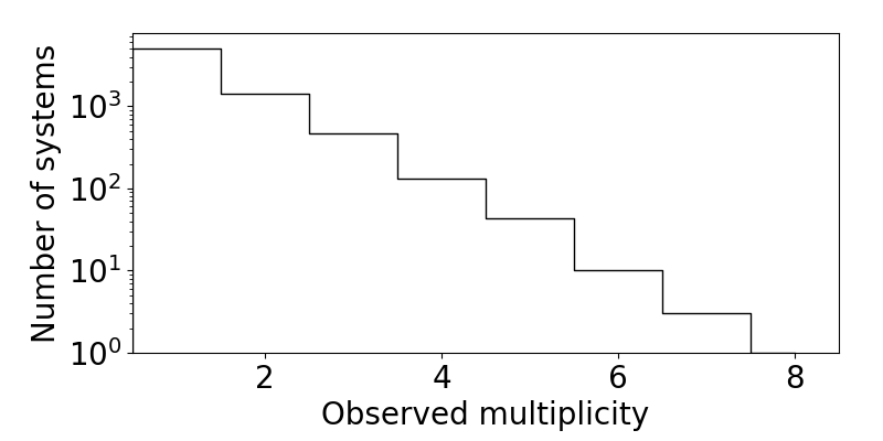
The observed multiplicity distribution of a simulated catalog.

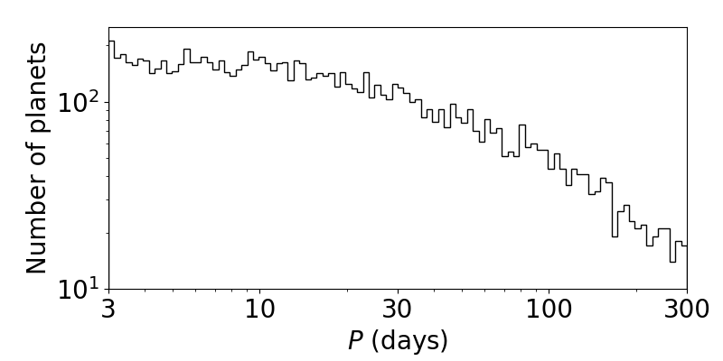
The observed period distribution of a simulated catalog.

As demonstrated above, the plot_fig_counts_hist_simple function should be used for quantities taking on discrete, integer values, as it is designed to center each bin on an integer. The multiplicity distribution is a perfect example of this case!

For continuous distributions (such as the period distribution), the plot_fig_pdf_simple function should be used.

Tip

The two functions above are actually wrappers of the functions plot_panel_counts_hist_simple and plot_panel_pdf_simple, respectively, which do most of the work and create a single panel (requiring an axes subplot object to plot on) instead of a figure. These are useful for making multi-panel figures!

Over-plotting the Kepler catalog

The third argument (empty list [] in the above examples) allows you to easily over-plot the Kepler catalog with a simulated observed catalog. Here is an example:

N_sim, cos_factor, P_min, P_max, radii_min, radii_max = read_targets_period_radius_bounds(load_dir + 'periods.out')

# Load the Kepler catalog first:
ssk_per_sys, ssk = compute_summary_stats_from_Kepler_catalog(P_min, P_max, radii_min, radii_max)

# To plot a histogram of the observed multiplicities (number of planets per system):
ax = plot_fig_counts_hist_simple([sss_per_sys['Mtot_obs']], [ssk_per_sys['Mtot_obs']], x_min=0, x_max=9, y_max=1, x_llim=0.5, normalize=True, log_y=True, xlabel_text='Observed multiplicity', ylabel_text='Fraction', legend=True)

# To plot a histogram of the observed orbital periods:
ax = plot_fig_pdf_simple([sss['P_obs']], [ssk['P_obs']], x_min=3., x_max=300., log_x=True, log_y=True, xticks_custom=[3,10,30,100,300], xlabel_text=r'$P$ (days)', legend=True)

plt.show()

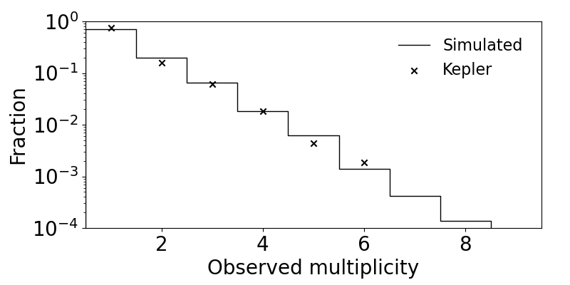
The observed multiplicity distribution of a simulated catalog compared to the Kepler catalog.

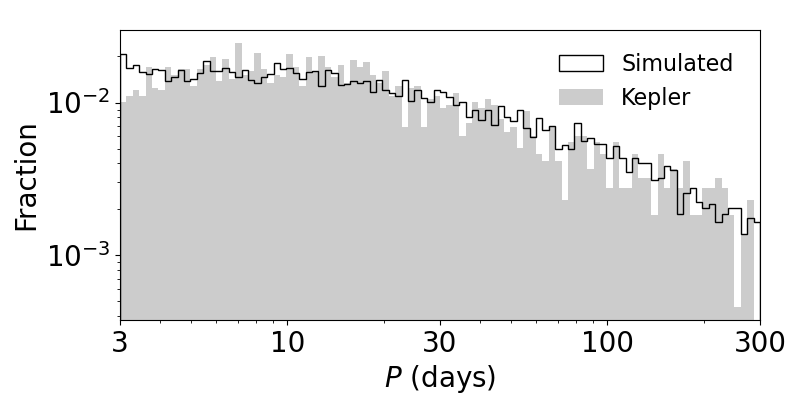
The observed period distribution of a simulated catalog compared to the Kepler catalog.

Note that we’ve set legend=True to tell which is which! The normalize=True option is also useful when the catalogs have different numbers of systems (in this case, the simulated catalog has five times as many targets as the Kepler catalog).

Plotting multiple catalogs

You can also plot multiple simulated (and Kepler) catalogs simultaneously by simply adding them to the lists:

Caution

The following example only works if you have more than one simulated catalog in the same folder (e.g. you downloaded the larger folder described in the “Downloading simulated catalogs” section), but it is illustrative of how easily you can do it.

# Load two separate simulated-observed catalogs,
# both of which are in the same 'load_dir',
# with run numbers '1' and '2'.
sss_per_sys1, sss1 = compute_summary_stats_from_cat_obs(file_name_path=load_dir, run_number='1')
sss_per_sys2, sss2 = compute_summary_stats_from_cat_obs(file_name_path=load_dir, run_number='2')

# To plot histograms of the observed orbital periods:
ax = plot_fig_pdf_simple([sss1['P_obs'], sss2['P_obs']], [], x_min=3., x_max=300., log_x=True, log_y=True, c_sim=['k','r'], ls_sim=['-','-'], labels_sim=['Catalog 1', 'Catalog 2'], xticks_custom=[3,10,30,100,300], xlabel_text=r'$P$ (days)', legend=True)

plt.show()

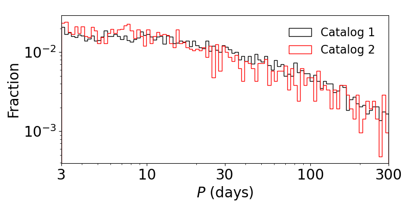
The observed period distributions of two simulated catalogs.

Note

You also need to pass lists for the optional arguments c_sim, ls_sim, and labels_sim to define the color, line-style, and legend label, respectively, for each catalog that you are plotting!

Plotting CDFs

Similarly, we also provide the following functions for plotting cumulative distribution functions (CDFs):

# To plot a CDF of the observed multiplicities:
ax = plot_fig_mult_cdf_simple([sss_per_sys['Mtot_obs']], [ssk_per_sys['Mtot_obs']], y_min=0.6, y_max=1., xlabel_text='Observed planets per system', legend=True)

# To plot a CDF of the observed orbital periods:
ax = plot_fig_cdf_simple([sss['P_obs']], [ssk['P_obs']], x_min=3., x_max=300., log_x=True, xticks_custom=[3,10,30,100,300], xlabel_text=r'$P$ (days)', legend=True)

plt.show()

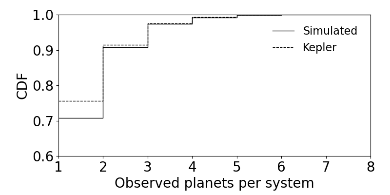
The observed multiplicity CDFs for a simulated and the Kepler catalog.

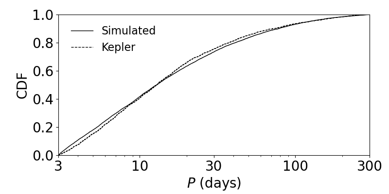
The observed period CDFs for a simulated and the Kepler catalog.